
The total angular momentum
 المؤلف:
Peter Atkins، Julio de Paula
المؤلف:
Peter Atkins، Julio de Paula
 المصدر:
ATKINS PHYSICAL CHEMISTRY
المصدر:
ATKINS PHYSICAL CHEMISTRY
 الجزء والصفحة:
ص348-351
الجزء والصفحة:
ص348-351
 2025-11-26
 28
28
The total angular momentum
One way of expressing the dependence of the spin–orbit interaction on the relative orientation of the spin and orbital momenta is to say that it depends on the total angular momentum of the electron, the vector sum of its spin and orbital momenta. Thus, when the spin and orbital angular momenta are nearly parallel, the total angular
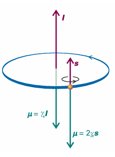
Fig. 10.26 Angular momentum gives rise to a magnetic moment (µ). For an electron, the magnetic moment is antiparallel to the orbital angular momentum, but proportional to it. For spin angular momentum, there is a factor 2, which increases the magnetic moment to twice its expected value (see Section 10.10).
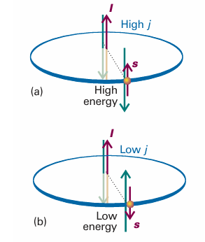
Fig. 10.27 Spin–orbit coupling is a magnetic interaction between spin and orbital magnetic moments. When the angular momenta are parallel, as in (a), the magnetic moments are aligned unfavourably; when they are opposed, as in (b), the interaction is favourable. This magnetic coupling is the cause of the splitting of a configuration into levels.
momentum is high; when the two angular momenta are opposed, the total angular momentum is low. The total angular momentum of an electron is described by the quantum numbers j and m j , with j = l + 1/2(when the two angular momenta are in the same direction) or j =l – 1/2(when they are opposed, Fig. 10.28). The different values of j that can arise for a given value of l label levels of a term. For l = 0, the only permitted value is j = 1/2 (the total angular momentum is the same as the spin angular momentum because there is no other source of angular momentum in the atom). When l = 1, j may be either 3/2 (the spin and orbital angular momenta are in the same sense) or 1/2 (the spin and angular momenta are in opposite senses).
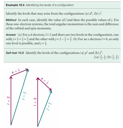
Fig. 10.28 The coupling of the spin and orbital angular momenta of a d electron (l = 2) gives two possible values of j depending on the relative orientations of the spin and orbital angular momenta of the electron.
The dependence of the spin–orbit interaction on the value of j is expressed in terms of the spin–orbit coupling constant, A (which is typically expressed as a wavenumber). A quantum mechanical calculation leads to the result that the energies of the levels with quantum numbers s, l, and j are given by
E l,s,j = 1/2hcA{j(j + 1) − l(l + 1) − s(s + 1)}
Justification 10.8 The energy of spin–orbit interaction
The energy of a magnetic moment µ in a magnetic field B is equal to their scalar product −µ ·B. If the magnetic field arises from the orbital angular momentum of the electron, it is proportional to l; if the magnetic moment µ is that of the electron spin, then it is proportional to s. It then follows that the energy of interaction is proportional to the scalar product s·l:
Energy of interaction =−µ ·B ∝ s·l We take this expression to be the first-order perturbation contribution to the hamiltonian. Next, we note that the total angular momentum is the vector sum of the spin and orbital momenta: j = l + s. The magnitude of the vector j is calculated by evaluating
j ·j = (l + s)·(l + s) = l·l + s·s + 2s·l
That is
s·l = 1/2{j2− l2− s2}
where we have used the fact that the scalar product of two vectors u and v is u·v = uv cos θ, from which it follows that u·u = u2. The preceding equation is a classical result. To make the transition to quantum mechanics, we treat all the quantities as operators, and write
s·l = 1/2{j2− l2− s2}
At this point, we calculate the first-order correction to the energy by evaluating the expectation value:

Then, by inserting this expression into the formula for the energy of interaction (E ∝ s·l), and writing the constant of proportionality as hcA/h2, we obtain eqn 10.42. The calculation of A is much more complicated: see Further reading.
llustration 10.3 Calculating the energies of levels
The unpaired electron in the ground state of an alkali metal atom has l = 0, so j = 1–2. Because the orbital angular momentum is zero in this state, the spin–orbit coup ling energy is zero (as is confirmed by setting j = s and l = 0 in eqn 10.41). When the electron is excited to an orbital with l = 1, it has orbital angular momentum and can give rise to a magnetic field that interacts with its spin. In this configuration the electron can have j = 3/2 or j = 1/2, and the energies of these levels are
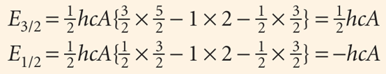
The corresponding energies are shown in Fig. 10.29. Note that the baricentre (the ‘centre of gravity’) of the levels is unchanged, because there are four states of energy 1/2hcA and two of energy −hcA.
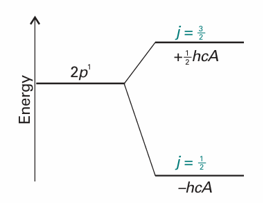
Fig. 10.29 The levels of a 2P term arising from spin–orbit coupling. Note that the low-j level lies below the high-j level in energy.
The strength of the spin–orbit coupling depends on the nuclear charge. To understand why this is so, imagine riding on the orbiting electron and seeing a charged nucleus apparently orbiting around us (like the Sun rising and setting). As a result, we find ourselves at the centre of a ring of current. The greater the nuclear charge, the greater this current, and therefore the stronger the magnetic field we detect. Because the spin magnetic moment of the electron interacts with this orbital magnetic field, it follows that the greater the nuclear charge, the stronger the spin–orbit interaction. The coupling increases sharply with atomic number (as Z4). Whereas it is only small in H (giving rise to shifts of energy levels of no more than about 0.4 cm−1), in heavy atoms like Pb it is very large (giving shifts of the order of thousands of reciprocal centimetres).
 الاكثر قراءة في مواضيع عامة في الكيمياء الفيزيائية
 اخر الاخبار
اخبار العتبة العباسية المقدسة


