

 تاريخ الرياضيات
 الرياضيات في الحضارات المختلفة
 الرياضيات المتقطعة
 الجبر
الجبر
 الهندسة
 المعادلات التفاضلية و التكاملية
 التحليل
 علماء الرياضيات
 |
Read More
Date: 19-4-2021
Date: 3-5-2021
Date: 9-3-2021
|
To show how histograms arise, and the associated parameters, we shall look at a few examples of rolling balanced dice and adding the results..
First, suppose one die is rolled. There are six possible outcomes, {1,2,3,4,5,6}, and if the die is balanced these six outcomes are equally likely—each has probability 1/6 . The histogram is very simple, and is shown in Fig. 1.1. The mean is

The median is also 1.1. The first quartile is 2 (we expect that a quarter of the rolls will be 2 or smaller). The easiest way to calculate this is that there are three equally

Fig. 1.1 Histograms for rolling one or two dice
likely values less than the mean, namely 1, 2 and 3; if we know that the roll will be less than 3.5, there are three possibilities, each with probability 1/3 , and the median of that set is 2. Similarly the third quartile is 5.
For the variance, the calculation is

and the standard deviation equals the square root of this, or approximately 1.71.
Say you roll two dice. For convenience, assume you can distinguish the two; maybe they are different colors, maybe you roll them separately. In any case, if you roll X on the first die and Y on the second, denote the result as XY. There are 36 possible rolls, 11, 12, 13, . . . , 66. Each of these results is equally likely with probability 1/36 .
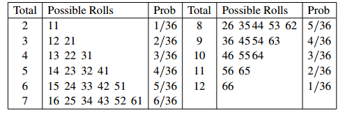
Usually, when rolling dice, you are interested in the total shown on the dice. As an example, the total 5 is obtained by the four rolls 14, 23, 32 and 41, and no others.
Each has probability 1/36 , and they are mutually exclusive, so the probability of a roll with total 5 is 4/36 or 1/9 . In the same way we can calculate the probability of every possible total: in the following table, Prob represents the probability of rolling a given total.

The histogram is also shown in Fig. 1.1. The mean and median are easily seen to be 7. (When the histogram is symmetric about some central value, it is easy to see that both mean and median will equal that central value.) The cumulative probability distribution is

Since 6/36 = 0.17 and 10/36 = 0.27 to two decimal places, the first quartile is 5; similarly, the third quartile is 9.
To two decimal places, the variance comes to 5.83, and the standard deviation is 2.42.
The case of three dice is handled similarly. There are 63 = 216 possible rolls. The probabilities of the different sums are

yielding a mean and median of 10.5 and quartiles 8 and 13. The variance comes to 8.75, and the standard deviation is approximately 2.96. The histogram is shown in Fig. 1.2.

Fig.1.2 Histogram for rolling three dice
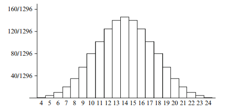
Finally, we consider rolling four dice. There are 64 = 1296 possible rolls, and the total can range from 4 to 24.


Fig. 1.3 Histogram for rolling four dice
with mean and median of 14 and quartiles 12 and 16. The variance is 11.666. . . , and the standard deviation is about 3.41. The histogram is shown in Fig. 1.3.


|
|
|
|
دراسة يابانية لتقليل مخاطر أمراض المواليد منخفضي الوزن
|
|
|
|
|
|
|
اكتشاف أكبر مرجان في العالم قبالة سواحل جزر سليمان
|
|
|
|
|
|
|
اتحاد كليات الطب الملكية البريطانية يشيد بالمستوى العلمي لطلبة جامعة العميد وبيئتها التعليمية
|
|
|