آخر المواضيع المضافة

 الفيزياء الكلاسيكية
الكهربائية والمغناطيسية
علم البصريات
الفيزياء الحديثة
النظرية النسبية
الفيزياء النووية
فيزياء الحالة الصلبة
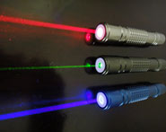
الليزر
علم الفلك
المجموعة الشمسية
الطاقة البديلة
الفيزياء والعلوم الأخرى
مواضيع عامة في الفيزياء
الفيزياء الكلاسيكية
الكهربائية والمغناطيسية
علم البصريات
الفيزياء الحديثة
النظرية النسبية
الفيزياء النووية
فيزياء الحالة الصلبة
الليزر
علم الفلك
المجموعة الشمسية
الطاقة البديلة
الفيزياء والعلوم الأخرى
مواضيع عامة في الفيزياء| Fourier Transform of the Autocorrelation Function |


|
|
Read More
Date: 15-9-2020
Date: 7-3-2016
Date: 15-12-2016
|
Fourier Transform of the Autocorrelation Function
Strictly, the Fourier transform is the end result or finished product of the Fourier integral. The transform is a continuous frequency-domain characterization of the strength of the wave feature (variance, amplitude, phase, etc.) over the continuum of frequencies. However, as applied to the autocorrelation function and in the discrete Fourier transform discussed below, it doesn't directly involve the Fourier integral. As a result, it's useful in many practical applications.
Stripped to its essentials, the method called the Fourier transform of the autocorrelation function consists of three steps:
1. Compute the autocorrelation of the time-series data, as described in the preceding chapter.
2. Transform the autocorrelation coefficients into the frequency domain. (There's an easy equation for this, e.g. Davis 1986: 260, eq. 4.102.)
3. "Smooth" the results to reduce noise and bring out any important frequencies.
Some people do the smoothing, discussed below, as step two rather than step three. That is, they smooth the autocorrelation coefficients rather than the variances or powers.
Historically, this method of getting frequency-domain information from a time series was the primary technique of Fourier analysis, especially in the several decades beginning in the 1950s. Davis (1986: 260) says that many people still use it. I'm not treating it in more detail here because in chaos analysis the more popular technique seems to be the discrete Fourier transform, discussed next.
|
|
|
|
التوتر والسرطان.. علماء يحذرون من "صلة خطيرة"
|
|
|
|
|
|
|
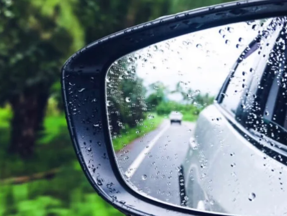
مرآة السيارة: مدى دقة عكسها للصورة الصحيحة
|
|
|
|
|
|
|
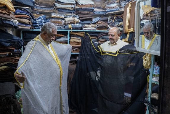
نحو شراكة وطنية متكاملة.. الأمين العام للعتبة الحسينية يبحث مع وكيل وزارة الخارجية آفاق التعاون المؤسسي
|
|
|