Tunnelling
If the potential energy of a particle does not rise to infinity when it is in the walls of the container, and E<v, the wavefunction does not decay abruptly to zero. If the walls are thin (so that the potential energy falls to zero again after a finite distance), then the wavefunction oscillates inside the box, varies smoothly inside the region representing the wall, and oscillates again on the other side of the wall outside the box (Fig. 9.9). Hence the particle might be found on the outside of a container even though according to classical mechanics it has insufficient energy to escape. Such leakage by penetration through a classically forbidden region is called tunnelling. The Schrödinger equation can be used to calculate the probability of tunnelling of a particle of mass mincident on a finite barrier from the left. On the left of the barrier (for x<0)
ψ=Aeikx+ Be−ikx kh=(2mE)1/2
The Schrödinger equation for the region representing the barrier (for 0 ≤x≤L), where the potential energy is the constant V, is
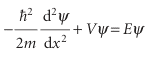
We shall consider particles that have E<v (so, according to classical physics, the particle has insufficient energy to pass over the barrier), and therefore V−E is positive. The general solutions of this equation are
ψ=Ceκx + De−κx κh={2m(V−E)}1/2
as we can readily verify by differentiating ψ twice with respect to x. The important feature to note is that the two exponentials are now real functions, as distinct from the complex, oscillating functions for the region where V=0 (oscillating functions would be obtained if E>V). To the right of the barrier (x>L), where V=0 again, the wave functions are
ψ=A′eikx + B′e−ikx k$ =(2mE)1/2
The complete wavefunction for a particle incident from the left consists of an incident wave, a wave reflected from the barrier, the exponentially changing amplitudes inside the barrier, and an oscillating wave representing the propagation of the particle to the right after tunnelling through the barrier successfully (Fig. 9.10). The acceptable wavefunctions must obey the conditions set out in Section 8.4b. In particular, they must be continuous at the edges of the barrier (at x = 0 and x = L, remembering that e0= 1):
A+B=C+D C eκL + De−κL =A′eikL + B′e−ikL
Their slopes (their first derivatives) must also be continuous there (Fig. 9.11):
ikA −ikB =κC−κD κCeκL −κDe−κL=ikA′eikL − ikB′e−ikL
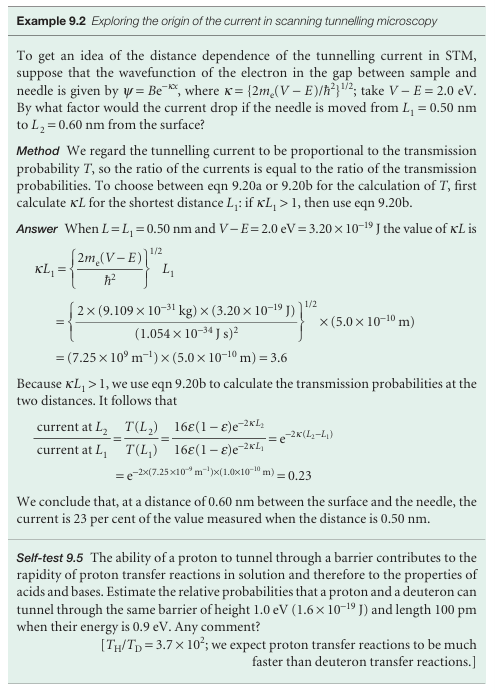
At this stage, we have four equations for the six unknown coefficients. If the particles are shot towards the barrier from the left, there can be no particles travelling to the left on the right of the barrier. Therefore, we can set B′=0, which removes one more unknown. We cannot set B = 0 because some particles may be reflected back from the barrier toward negative x. The probability that a particle is travelling towards positive x (to the right) on the left of the barrier is proportional to | A |2, and the probability that it is travelling to the right on the right of the barrier is | A′|2. The ratio of these two probabilities is called the transmission probability, T. After some algebra (see Problem 9.9) we find

where ε = E/V. This function is plotted in Fig. 9.12; the transmission coefficient for E>Vis shown there too. For high, wide barriers (in the sense that κL >> 1), eqn 9.20a simplifies to
T≈16ε(1−ε) e−2κL
The transmission probability decreases exponentially with the thickness of the barrier and with m1/2. It follows that particles of low mass are more able to tunnel through barriers than heavy ones (Fig. 9.13). Tunnelling is very important for electrons and muons, and moderately important for protons; for heavier particles it is less important.
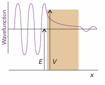
Fig. 9.9A particle incident on a barrier from the left has an oscillating wave function, but inside the barrier there are no oscillations (for E<v). If the barrier is not too thick, the wavefunction is nonzero at its opposite face, and so oscillates begin again there. (Only the real component of the wavefunction is shown.)
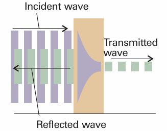
Fig. 9.10 When a particle is incident on a barrier from the left, the wavefunction consists of a wave representing linear momentum to the right, a reflected component representing momentum to the left, a varying but not oscillating component inside the barrier, and a (weak) wave representing motion to the right on the far side of the barrier.
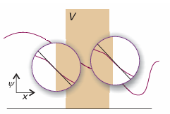
Fig. 9.11 The wavefunction and its slope must be continuous at the edges of the barrier. The conditions for continuity enable us to connect the wavefunctions in the three zones and hence to obtain relations between the coefficients that appear in the solutions of the Schrödinger equation.
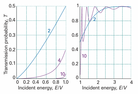
Fig. 9.12 The transition probabilities for passage through a barrier. The horizontal axis is the energy of the incident particle expressed as a multiple of the barrier height. The curves are labelled with the value of L(2mV)1/2/$. The graph on the left is for E < V and that on the right for E > V. Note that T > 0 for E < V whereas classically T would be zero. However, T < 1 for E > V, whereas classically T would be 1.
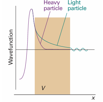
Fig. 9.13 The wavefunction of a heavy particle decays more rapidly inside a barrier than that of a light particle. Consequently, a light particle has a greater probability of tunnelling through the barrier.
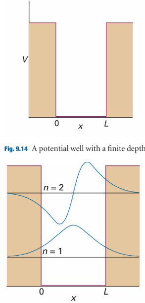
Fig. 9.15 The lowest two bound-state wavefunctions for a particle in the well shown in Fig. 9.14 and one of the wavefunctions corresponding to an unbound state (E > V).
A number of effects in chemistry (for example, the isotope-dependence of some reaction rates) depend on the ability of the proton to tunnel more readily than the deuteron. The very rapid equilibration of proton transfer reactions is also a mani festation of the ability of protons to tunnel through barriers and transfer quickly from an acid to a base. Tunnelling of protons between acidic and basic groups is also an important feature of the mechanism of some enzyme-catalysed reactions. As we shall see in Chapters 24 and 25, electron tunnelling is one of the factors that determine the rates of electron transfer reactions at electrodes and in biological systems. A problem related to the one just considered is that of a particle in a square-well potential of finite depth (Fig. 9.14). In this kind of potential, the wavefunction penetrates into the walls, where it decays exponentially towards zero, and oscillates within the well. The wavefunctions are found by ensuring, as in the discussion of tunnelling, that they and their slopes are continuous at the edges of the potential. Some of the lowest energy solutions are shown in Fig. 9.15. A further difference from the solutions for an infinitely deep well is that there is only a finite number of bound states. Regardless of the depth and length of the well, there is always at least one bound state. Detailed consideration of the Schrödinger equation for the problem shows that in general the number of levels is equal to N, with

where Vis the depth of the well and L is its length (for a derivation of this expression, see Further reading). We see that the deeper and wider the well, the greater the number of bound states. As the depth becomes infinite, so the number of bound states also becomes infinite, as we have already seen.
Nanoscience is the study of atomic and molecular assemblies with dimensions ranging from 1 nm to about 100 nm and nanotechnology is concerned with the incorporation of such assemblies into devices. The future economic impact of nanotechnology could be very significant. For example, increased demand for very small digital electronic devices has driven the design of ever smaller and more powerful microprocessors. However, there is an upper limit on the density of electronic circuits that can be incorporated into silicon-based chips with current fabrication technologies. As the ability to process data increases with the number of circuits in a chip, it follows that soon chips and the devices that use them will have to become bigger if processing power is to increase indefinitely. One way to circumvent this problem is to fabricate devices from nanometre-sized components. We will explore several concepts of nanoscience throughout the text. We begin with the description of scanning probe microscopy (SPM), a collection of techniques that can be used to visualize and manipulate objects as small as atoms on surfaces. Consequently, SPM has far better resolution than electron microscopy (Impact I8.1). One modality of SPM is scanning tunnelling microscopy (STM), in which a platinum rhodium or tungsten needle is scanned across the surface of a conducting solid. When the tip of the needle is brought very close to the surface, electrons tunnel across the intervening space (Fig. 9.16). In the constant-current mode of operation, the stylus moves up and down corresponding to the form of the surface, and the topography of the surface, including any adsorbates, can be mapped on an atomic scale. The vertical motion of the stylus is achieved by fixing it to a piezoelectric cylinder, which contracts or expands according to the potential difference it experiences. In the constant-z mode, the vertical position of the stylus is held constant and the current is monitored. Because the tunnelling probability is very sensitive to the size of the gap, the micro scope can detect tiny, atom-scale variations in the height of the surface. Figure 9.17 shows an example of the kind of image obtained with a surface, in this case of gallium arsenide, that has been modified by addition of atoms, in this case caesium atoms. Each ‘bump’ on the surface corresponds to an atom. In a further variation of the STM technique, the tip may be used to nudge single atoms around on the surface, making possible the fabrication of complex and yet very tiny nanometre sized structures. In atomic force microscopy (AFM) a sharpened stylus attached to a cantilever is scanned across the surface. The force exerted by the surface and any bound species pushes or pulls on the stylus and deflects the cantilever (Fig. 9.18). The deflection is monitored either by interferometry or by using a laser beam. Because no current is needed between the sample and the probe, the technique can be applied to non-conducting surfaces too. A spectacular demonstration of the power of AFM is given in Fig. 9.19, which shows individual DNA molecules on a solid surface.
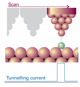
Fig. 9.16 A scanning tunnelling microscope makes use of the current of electrons that tunnel between the surface and the tip. That current is very sensitive to the distance of the tip above the surface.
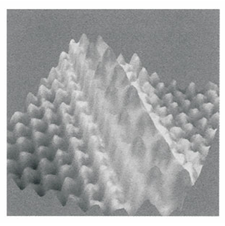
Fig. 9.17 An STM image of caesium atoms on a gallium arsenide surface.
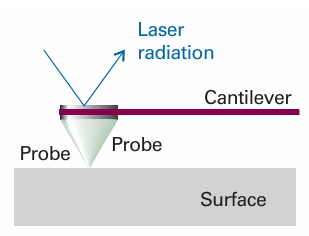
Fig. 9.18 In atomic force microscopy, a laser beam is used to monitor the tiny changes in the position of a probe as it is attracted to or repelled from atoms on a surface.
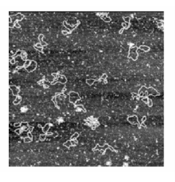
Fig. 9.19 An AFM image of bacterial DNA plasmids on a mica surface. (Courtesy of Veeco Instruments.)
 الاكثر قراءة في مواضيع عامة في الكيمياء الفيزيائية
 اخر الاخبار
اخبار العتبة العباسية المقدسة


