we have obtained the converse R˘ of R by turning around all the arrows, resp. the order of the components. This was always possible, since a relation was just a set of ordered pairs with no other conditions attached.

For a function, reversing the arrows need not result in another function: Consider the examples in Figure 1.1in ( One–one, Onto, and Bijective Functions)  . In the surjective function, turning around the arrows does not result in a function, because there are two arrows leaving e.

Furthermore, you will notice that applying f to an element of dom f and then applying g to the result gets us right back to where we started, in other words,  g(f(a)) = a. This property is decisive, and leads to the following

Definition 1.1. Let f : A → B and g : B → A be functions; g is called the inverse of f, denoted by f⁻¹ , if g(f(x)) = x for all x ∈ A.

In other words, g is an inverse of f if and only if g ◦ f = idA. The examples above suggest that a function which is not bijective cannot have an inverse. The following Theorem shows that this observation is correct.

Theorem 1.1. f : A → B has an inverse if and only if f is injective.

Proof. “⇒”: Suppose that g : B → A is an inverse of f; we have to show that f is one–one. Let x,y ∈ A and f(x) = f(y); then, g(f(x)) = g(f(y)). Since g is an inverse of f, we have g(f(x)) = x and g(f(y)) = y, which implies x = y.

“⇐”: Suppose that f : A → B is one–one; for each y ∈ B we distinguish two cases:

1. y ∈ ran f: Then there is exactly one x ∈ A such that f(x) = y, since f is one–one. Now set g(y) = x.

2. x ∉ran f: Choose an arbitrary element yx of A, and set g(y) = yx. So,  dom g = B, codom g = A, and, since, f is one–one, each element of B is assigned exactly one element of A; hence, g : B → A is a function.

Finally, let x ∈ A; by definition of g we have g(f(x)) = x, which shows that g is an inverse of f.

Note that in case f is one–one but not onto it has more than one inverse function,  since g is defined arbitrarily for every x ∈ B which is not in the range of f. Those elements of the codomain which are not in the range of f are in a way immaterial to the assignment f; from previous examples we know that a one–one function can be made bijective by restricting its codomain to the range. If f is bijective then there is only one inverse function:

Theorem 1.2. If f : A → B is bijective, then f has unique inverse g : B → A;  furthermore, f is an inverse to g.

Proof. Since f is bijective, it is one–one, and thus it has an inverse g : B → A.

Suppose that h : B → A is also an inverse to f, i.e. we have h(f(x)) = x for every x ∈ A. Since in particular f is onto, for every y ∈ B there is an x ∈ A such that f(x) = y; now, since g is an inverse to f, we have g(y) = g(f(x)) = x,  and since h is also an inverse to f, we have h(y) = h(f(x)) = x. It follows that g(y) = h(y) for all y ∈ B, which shows that g = h.

For the second part we have to show that f(g(y)) = y for all y B. Thus, let y ∈ B.

Since f is onto, there exists an x ∈ A such that f(x) = y. Thus,

                f(g(y)) = f(g(f(x))) = f(x),

since g is an inverse of f, and hence, g(f(x)) = x.

Let us briefly look at bijective functions f : A → A, where A is a finite set.

Definition 1.2. Let A = {1, 2, 3,. . ., n}, and f : A → A be a bijective function;

then f is called a permutation on n.

The reason for calling these function permutations is that they arrange (i.e. permute)  the elements of Ain a different order. Amore general definition of a permutation would allow as domain arbitrary finite sets. For example, if you have n books arranged on a shelf and you put them in a different order, you have in fact performed a permutation of n objects.

If n is small there is a convenient way of picturing f; for example if A = {1, 2, 3, 4, 5}, and f(1) = 1, f(2) = 3, f(3) = 5, f(4) = 2, f(5) = 4, then we can write

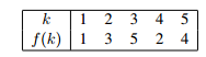
Observe that every element of A appears exactly once in each of the two lines,  since f is bijective. In general, if A = {1, 2,. . ., n}, and f(1) = a₁,f(2) = a₂,. . ., f(n) = a_n, we can list the function by

It is easy to find the inverse of a permutation by just looking from bottom to top in the given list. Let us go back to the example above: The inverse g of f looks like this:

This method of representing a permutation is also useful for obtaining the composition;  look at the following two permutations of A:

By going through the tables, we find that for h = g ◦ f,

اخر الاخبار

اخبار العتبة العباسية المقدسة

عباس.. طفل فقد والده فوجد في خدمة زائري عاشوراء وطنًا آمنًا

شعبة الخطابة النسوية تواصل إقامة مجالس العزاء في شهر المحرم الحرام

لليوم الخامس.. العتبة العباسية المقدسة تقيم مجلس عزاء في صحن مرقد أبي الفضل العباس (عليه السلام)

قسم الشؤون الفكرية يقيم مجلس عزاء حسيني في العاصمة التنزانية دار السلام

المزيد

الآخبار الصحية

لمن تجاوز الستين.. عليك بشرب 4 أكواب من القهوة يوميا ؟

الحليب مع العسل.. مزيج يمنحك 7 فوائد صحية

لا تبالغ في التنظيف.. قليل من "الاتساخ" قد يحمي عائلتك

دراسة تكشف علاقة خطيرة بين عمر الأم وصحة مولودها

المزيد

الآخبار التكنلوجية

هل هاتفك مراقب؟.. 5 علامات خطيرة تكشف التجسس عليك

دبي تطلق أول رحلة تجريبية للتاكسي الجوي

كيف تساعد الصيانة الوقائية في الحفاظ على كفاءة التكييف في سيارتك ؟

في ظاهرة غريبة حيرت العلماء.. كوكبنا قد يسجل أقصر يوم في التاريخ هذا الصيف!

المزيد

مواضيع ذات صلة

Subset

Set Class

Set

Second Category

Proper Subset

Power Set

Matroid

Inductive Set

Independent Vertex Set

Independent Set

Graphoid

G_delta Set