

تاريخ الرياضيات

الاعداد و نظريتها

تاريخ التحليل

تار يخ الجبر

الهندسة و التبلوجي


الرياضيات في الحضارات المختلفة

العربية

اليونانية

البابلية

الصينية

المايا

المصرية

الهندية


الرياضيات المتقطعة

المنطق

اسس الرياضيات

فلسفة الرياضيات

مواضيع عامة في المنطق


الجبر

الجبر الخطي

الجبر المجرد

الجبر البولياني

مواضيع عامة في الجبر

الضبابية

نظرية المجموعات

نظرية الزمر

نظرية الحلقات والحقول

نظرية الاعداد

نظرية الفئات

حساب المتجهات

المتتاليات-المتسلسلات

المصفوفات و نظريتها

المثلثات


الهندسة

الهندسة المستوية

الهندسة غير المستوية

مواضيع عامة في الهندسة

التفاضل و التكامل


المعادلات التفاضلية و التكاملية

معادلات تفاضلية

معادلات تكاملية

مواضيع عامة في المعادلات


التحليل

التحليل العددي

التحليل العقدي

التحليل الدالي

مواضيع عامة في التحليل

التحليل الحقيقي

التبلوجيا

نظرية الالعاب

الاحتمالات و الاحصاء

نظرية التحكم

بحوث العمليات

نظرية الكم

الشفرات

الرياضيات التطبيقية

نظريات ومبرهنات


علماء الرياضيات

500AD

500-1499

1000to1499

1500to1599

1600to1649

1650to1699

1700to1749

1750to1779

1780to1799

1800to1819

1820to1829

1830to1839

1840to1849

1850to1859

1860to1864

1865to1869

1870to1874

1875to1879

1880to1884

1885to1889

1890to1894

1895to1899

1900to1904

1905to1909

1910to1914

1915to1919

1920to1924

1925to1929

1930to1939

1940to the present

علماء الرياضيات

الرياضيات في العلوم الاخرى

بحوث و اطاريح جامعية

هل تعلم

طرائق التدريس

الرياضيات العامة

نظرية البيان
THE PONTRYAGIN MAXIMUM PRINCIPLE-APPLICATIONS AND EXAMPLES
المؤلف:
Lawrence C. Evans
المصدر:
An Introduction to Mathematical Optimal Control Theory
الجزء والصفحة:
50-59
9-10-2016
2110
HOW TO USE THE MAXIMUM PRINCIPLE. We mentioned earlier that the costate p∗(.) can be interpreted as a sort of Lagrange multiplier.
Calculations with Lagrange multipliers. Recall our discussion in (REVIEW OF LAGRANGE MULTIPLIERS)about finding a point x∗ that maximizes a function f, subject to the requirement that g ≤ 0. Now x∗ = (x∗1, . . . , x∗n)T has n unknown components we must find.
Somewhat unexpectedly, it turns out in practice to be easier to solve (1.4) for the n + 1 unknowns x∗1, . . . , x∗n and λ. We repeat this key insight: it is actually easier to solve the problem if we add a new unknown, namely the Lagrange multiplier.
Worked examples abound in multivariable calculus books.
Calculations with the costate. This same principle is valid for our much more complicated control theory problems: it is usually best not just to look for an optimal control α∗(.) and an optimal trajectory x∗(.) alone, but also to look as well for the costate p∗(.). In practice, we add the equations (ADJ) and (M) to (ODE) and then try to solve for α∗(.), x∗(.) and for p∗(.).
The following examples show how this works in practice, in certain cases for which we can actually solve everything explicitly or, failing that, at least deduce some useful information.
EXAMPLE 1: LINEAR TIME-OPTIMAL CONTROL. For this example, let A denote the cube [−1, 1] n in Rn. We consider again the linear dynamics:

for the payoff functional

where τ denotes the first time the trajectory hits the target point x1 = 0. We have r ≡ −1, and so
H(x, p, a) = f . p + r = (Mx + Na) . p − 1.
1.2 EXAMPLE 2: CONTROL OF PRODUCTION AND CONSUMPTION. We return to Example 1 in INTRODUCTION, a model for optimal consumption in a simple economy. Recall that
x(t) = output of economy at time t,
α(t) = fraction of output reinvested at time t.
We have the constraint 0 ≤ α(t) ≤ 1; that is, A = [0, 1] ⊂ R. The economy evolves according to the dynamics

where x0 > 0 and we have set the growth factor k = 1. We want to maximize the total consumption

How can we characterize an optimal control α∗(.)?
Introducing the maximum principle. We apply Pontryagin Maximum Principle, and to simplify notation we will not write the superscripts ∗ for the optimal control, trajectory, etc. We have n = m = 1,
f(x, a) = xa, g ≡ 0, r(x, a) = (1 − a)x;
and therefore
H(x, p, a) = f(x, a)p + r(x, a) = pxa + (1 − a)x = x + ax(p − 1).
The dynamical equation is

and the adjoint equation is

The terminal condition reads
(T) p(T) = gx(x(T)) = 0.
Lastly, the maximality principle asserts

Using the maximum principle. We now deduce useful information from (ODE), (ADJ), (M) and (T).
According to (M), at each time t the control value α(t) must be selected to maximize a(p(t) − 1) for 0 ≤ a ≤ 1. This is so, since x(t) > 0. Thus

Hence if we know p(.), we can design the optimal control α(.).
So next we must solve for the costate p(.). We know from (ADJ) and (T) that

Since p(T) = 0, we deduce by continuity that p(t) ≤ 1 for t close to T, t < T. Thus α(t) = 0 for such values of t. Therefore ˙ p(t) = −1, and consequently p(t) = T – t for times t in this interval. So we have that p(t) = T − t so long as p(t) ≤ 1. And this holds for T − 1 ≤ t ≤ T But for times t ≤ T − 1, with t near T − 1, we have α(t) = 1; and so (ADJ) becomes

Since p(T − 1) = 1, we see that p(t) = eT−1−t> 1 for all times 0 ≤ t ≤ T − 1. In particular there are no switches in the control over this time interval.
Restoring the superscript * to our notation, we consequently deduce that an optimal control is

for the optimal switching time t∗ = T − 1.
We leave it as an exercise to compute the switching time if the growth constant k = 1.
1.3 EXAMPLE 3: A SIMPLE LINEAR-QUADRATIC REGULATOR. We take n = m = 1 for this example, and consider the simple linear dynamics

with the quadratic cost functional

which we want to minimize. So we want to maximize the payoff functional

For this problem, the values of the controls are not constrained; that is, A = R.
Introducing the maximum principle. To simplify notation further we again drop the superscripts ∗. We have n = m = 1,
f(x, a) = x + a, g ≡ 0, r(x, a) = −x2− a2;
and hence
H(x, p, a) = fp + r = (x + a)p − (x2+ a2)
The maximality condition becomes

We calculate the maximum on the right hand side by setting Ha = −2a + p = 0.
Thus a = p/2 , and so

The dynamical equations are therefore

Moreover x(0) = x0 , and the terminal condition is (T) p(T) = 0.
Using the Maximum Principle. So we must look at the system of equations

the general solution of which is

Since we know x0, the task is to choose p0 so that p(T) = 0.
Feedback controls. An elegant way to do so is to try to find optimal control in linear feedback form; that is, to look for a function c(.) : [0, T] → R for which α(t) = c(t) x(t).
We henceforth suppose that an optimal feedback control of this form exists, and attempt to calculate c(.). Now

We will next discover a differential equation that d(.) satisfies. Compute

Since p(T) = 0, the terminal condition is d(T) = 0.
So we have obtained a nonlinear first–order ODE for d(.) with a terminal boundary condition:

This is called the Riccati equation.
In summary so far, to solve our linear–quadratic regulator problem, we need to first solve the Riccati equation (R) and then set

How to solve the Riccati equation. It turns out that we can convert (R) it into a second–order, linear ODE. To accomplish this, write

for a function b(.) to be found. What equation does b(.) solve? We compute

This is a terminal-value problem for second–order linear ODE, which we can solve by standard techniques. We then set d = 2b˙ / b , to derive the solution of the Riccati equation (R).
We will generalize this example later to systems
1.4 EXAMPLE 4: MOON LANDER. This is a much more elaborate and interesting example, already introduced in INTRODUCTION. We follow the discussion of Fleming and Rishel [F-R].
Introduce the notation
h(t) = height at time t
v(t) = velocity = ˙ h(t)
m(t) = mass of spacecraft (changing as fuel is used up)
α(t) = thrust at time t.
The thrust is constrained so that 0 ≤ α(t) ≤ 1; that is, A = [0, 1]. There are also the constraints that the height and mass be nonnegative: h(t) ≥ 0,m(t) ≥ 0.
The dynamics are

with initial conditions
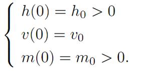
The goal is to land on the moon safely, maximizing the remaining fuel m(τ ), where τ = τ [α()] is the first time h(τ ) = v(τ ) = 0. Since α = − m˙/ k , our intention is equivalently to minimize the total applied thrust before landing; so that

Introducing the maximum principle. In terms of the general notation, we have

Hence the Hamiltonian is

We next have to figure out the adjoint dynamics (ADJ). For our particular Hamiltonian,

Therefore

The maximization condition (M) reads
(M)

Thus the optimal control law is given by the rule:

Using the maximum principle. Now we will attempt to figure out the form of the solution, and check it accords with the Maximum Principle.
Let us start by guessing that we first leave rocket engine of (i.e., set α ≡ 0) and turn the engine on only at the end. Denote by τ the first time that h(τ ) = v(τ ) = 0, meaning that we have landed. We guess that there exists a switching time t∗ < τ when we turned engines on at full power (i.e., set α ≡ 1).Consequently,

Therefore, for times t∗ ≤ t ≤ τ our ODE becomes

Suppose the total amount of fuel to start with was m1; so that m0 −m1 is the weight of the empty spacecraft. When α ≡ 1, the fuel is used up at rate k. Hence
k(τ − t∗) ≤ m1,

Before time t∗, we set α ≡ 0. Then (ODE) reads
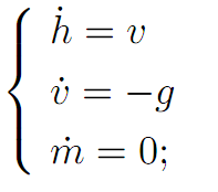
and thus
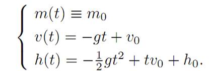
We combine the formulas for v(t) and h(t), to discover

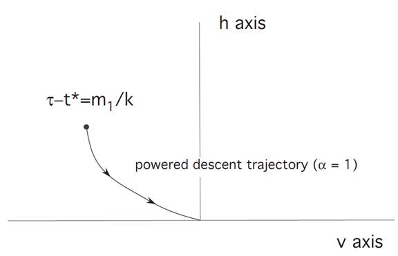
We deduce that the freefall trajectory (v(t), h(t)) therefore lies on a parabola
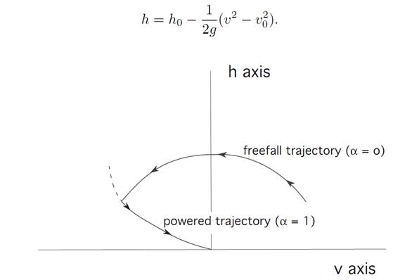
If we then move along this parabola until we hit the soft-landing curve from the previous picture, we can then turn on the rocket engine and land safely.
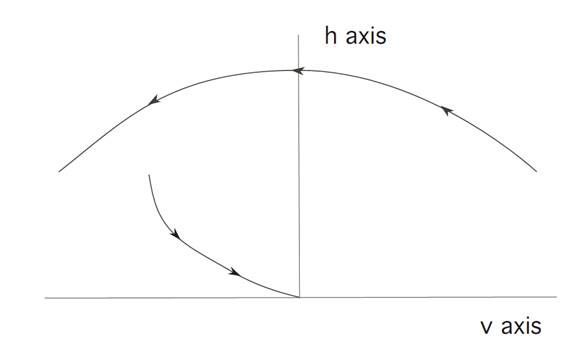
In the second case illustrated, we miss switching curve, and hence cannot land safely on the moon switching once.
To justify our guess about the structure of the optimal control, let us now find the costate p(.) so that α(.) and x(.) described above satisfy (ODE), (ADJ), (M).
To do this, we will have have to figure out appropriate initial conditions
p1 (0) = λ1, p2 (0) = λ2, p3 (0) = λ3.
We solve (ADJ) for α(.) as above, and find
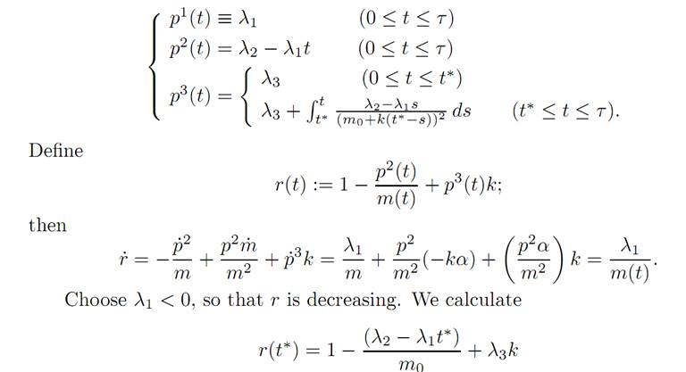
and then adjust λ2, λ3 so that r(t∗) = 0.
Then r is nonincreasing, r(t∗) = 0, and consequently r > 0 on [0, t∗), r < 0 on (t∗, τ ]. But (M) says

Thus an optimal control changes just once from 0 to 1; and so our earlier guess of α(.) does indeed satisfy the Pontryagin Maximum Principle.
References
[B-CD] M. Bardi and I. Capuzzo-Dolcetta, Optimal Control and Viscosity Solutions of Hamilton-Jacobi-Bellman Equations, Birkhauser, 1997.
[B-J] N. Barron and R. Jensen, The Pontryagin maximum principle from dynamic programming and viscosity solutions to first-order partial differential equations, Transactions AMS 298 (1986), 635–641.
[C1] F. Clarke, Optimization and Nonsmooth Analysis, Wiley-Interscience, 1983.
[C2] F. Clarke, Methods of Dynamic and Nonsmooth Optimization, CBMS-NSF Regional Conference Series in Applied Mathematics, SIAM, 1989.
[Cr] B. D. Craven, Control and Optimization, Chapman & Hall, 1995.
[E] L. C. Evans, An Introduction to Stochastic Differential Equations, lecture notes avail-able at http://math.berkeley.edu/˜ evans/SDE.course.pdf.
[F-R] W. Fleming and R. Rishel, Deterministic and Stochastic Optimal Control, Springer, 1975.
[F-S] W. Fleming and M. Soner, Controlled Markov Processes and Viscosity Solutions, Springer, 1993.
[H] L. Hocking, Optimal Control: An Introduction to the Theory with Applications, OxfordUniversity Press, 1991.
[I] R. Isaacs, Differential Games: A mathematical theory with applications to warfare and pursuit, control and optimization, Wiley, 1965 (reprinted by Dover in 1999).
[K] G. Knowles, An Introduction to Applied Optimal Control, Academic Press, 1981.
[Kr] N. V. Krylov, Controlled Diffusion Processes, Springer, 1980.
[L-M] E. B. Lee and L. Markus, Foundations of Optimal Control Theory, Wiley, 1967.
[L] J. Lewin, Differential Games: Theory and methods for solving game problems with singular surfaces, Springer, 1994.
[M-S] J. Macki and A. Strauss, Introduction to Optimal Control Theory, Springer, 1982.
[O] B. K. Oksendal, Stochastic Differential Equations: An Introduction with Applications, 4th ed., Springer, 1995.
[O-W] G. Oster and E. O. Wilson, Caste and Ecology in Social Insects, Princeton UniversityPress.
[P-B-G-M] L. S. Pontryagin, V. G. Boltyanski, R. S. Gamkrelidze and E. F. Mishchenko, The Mathematical Theory of Optimal Processes, Interscience, 1962.
[T] William J. Terrell, Some fundamental control theory I: Controllability, observability, and duality, American Math Monthly 106 (1999), 705–719.
 الاكثر قراءة في نظرية التحكم
 اخر الاخبار
اخبار العتبة العباسية المقدسة

الآخبار الصحية


 قسم الشؤون الفكرية يصدر كتاباً يوثق تاريخ السدانة في العتبة العباسية المقدسة
 "المهمة".. إصدار قصصي يوثّق القصص الفائزة في مسابقة فتوى الدفاع المقدسة للقصة القصيرة
 (نوافذ).. إصدار أدبي يوثق القصص الفائزة في مسابقة الإمام العسكري (عليه السلام)


