

 تاريخ الرياضيات
 الرياضيات في الحضارات المختلفة
 الرياضيات المتقطعة
 الجبر
الجبر
 الهندسة
 المعادلات التفاضلية و التكاملية
 التحليل
 علماء الرياضيات
 |
Read More
Date: 31-3-2021
Date: 6-2-2021
Date: 12-4-2021
|
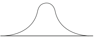
In many cases, the histogram of a probability distribution looks like the bell-shaped curve shown in Fig. 1.1. In that case, the curve is called a normal curve and the distribution is called a normal distribution. The curve extends infinitely far in both directions, but the probability of an extreme value is very small.
Some simple probability distributions are close to the normal distribution. In general, when there are a number of different factors added together to give the value of the event, the distribution is close to the normal. For example, the heights of adults are approximately normal. They obviously do not follow a normal distribution exactly—the probability of a negative height is zero—but the distribution is very close to the normal. We commonly say a variable is “distributed normally” when the distribution is close to normal, even if not exactly normal. One important example is that nearly all sample means are approximately normal. After all, you calculate the mean by adding a number of different factors—the different values of the variable in the sample—before you divide by the number of members. So the properties of the normal distribution can be used in analyzing sample means.

Fig. 1.1 The normal curve
The histogram of the normal distribution is a symmetric bell-shaped curve. The precise shape depends on the amount of spread, which is most commonly measured by the standard deviation. Suppose the mean is µ and the standard deviation is σ.
Then the center of the curve, its highest point, is at µ, the mean, which also equals the median and the mode.
In a normal distribution, approximately 68.2689% of the scores will lie in the range from µ − σ to µ + σ. In other words, the probability that a reading lies between µ−σ and µ+σ is about 68%, or 0.68 if you prefer. (For our purposes, it is usually sufficient to give probabilities to the nearest percentage.) The first quartile is approximately µ − 2/3σ, and the third quartile is approximately µ + 2/3σ.
As an example, suppose the weights of 1-year-old children in your city average 25 lbs, and the standard deviation of weights is 3 lbs. (These are approximations of the figures for 1-year-olds in the United States, as given by National Health Statistics; in the real world, the standard deviation is a little larger.) The weights of children of a given age are very close to a normal distribution. So we would expect that about 68% of the 1-year-old children in the city weigh between 22 and 28 lbs. The normal histogram is symmetric about the mean, so we would expect 34% to lie between 22 and 25 lbs, and another 34% between 25 and 28. The first quartile is 23, so about one-fourth of 1-year-olds weigh less than 23 lbs, another fourth are between 23 and 25, and so on.
About 95% of the scores in a normal distribution lie within two standard deviations of the mean—between µ−2σ and µ+2σ—so (using the symmetry) there are 2.5% of scores greater than µ + 2σ, and the same number less than µ − 2σ. So among the 1-year-olds, all but 5% would have weights in the range from 19 to 31 lbs.
Sample Problem 1.1 Assume the height of women in the United States is normally distributed with mean 64 in and standard deviation 2.4 in. Find ranges that contain the heights of the middle 68% of all United States women and the middle 95% of all women.
Solution. The middle 68% of scores in a normal distribution with mean µ and standard deviation σ lie between µ − σ and µ + σ. So 68% of women’s heights lie between 61.6 and 66.4 in. The formula for 95% uses 2σ instead of σ, so the range is 59.2–68.8 in.
The facts that 68% of scores lie in the range µ ±σ and 95% in the range µ ±2σ is called the 68–95 rule for normal distributions, and is illustrated in Fig. 1.2.
Since 68% or scores lie in the range µ±σ, there are 32% outside that range. Half (16%) will be greater and half will be smaller. So 16% of readings lie above µ + σ and another 16% lie below µ − σ. Similarly 2.5% are above µ + 2σ and 2.5% are below µ −2σ.
Sample Problem 1.2 Given the data in the preceding Sample Problem, how many US women are taller than 68.8 in?
Solution. As 68.8 in is µ +2σ, 2.5% of women are taller.

Fig. 1.2 68–95 rule
The percentage that lie within three standard deviations of the mean is about 99.7%, and the corresponding percentage for four standard deviations is a little greater than 99.99%.
If you look at the histograms for rolling dice that we constructed in the preceding section, you will see that the more dice you roll, the more the histogram looks like a normal curve.


|
|
|
|
التوتر والسرطان.. علماء يحذرون من "صلة خطيرة"
|
|
|
|
|
|
|
مرآة السيارة: مدى دقة عكسها للصورة الصحيحة
|
|
|
|
|
|
|
نحو شراكة وطنية متكاملة.. الأمين العام للعتبة الحسينية يبحث مع وكيل وزارة الخارجية آفاق التعاون المؤسسي
|
|
|